Intermediates 🤓🤓 Featured

From HuggingFace dataset to Qdrant vector database in 12 minutes flat

In this tutorial, we will transform a dataset from the HuggingFace Hub into a Qdrant vector database in 12 minutes flat (for free).

Mary Newhauser

Jan 26, 2024 • 7 min read

Image by the author.

Using a vector database with a robust Python client, like Qdrant, is a simple, cheap, and effective way to leverage large text datasets, saving their embeddings for future downstream tasks.

This tutorial will demonstrate how to transform a text-based dataset from the HuggingFace Hub into a local Qdrant vector database, using Sentence Transformers and a free Google Colab GPU-enabled notebook. We will go over how to set up your Google Colab notebook, load an existing dataset from the HuggingFace Hub, generate sentence embeddings using the small (but robust) all-MiniLM-L6-v2 model, upsert the embeddings into a local Qdrant database, and finally query the embedded text and explore the dataset.

And as the title promises, we can complete the entire project in just 12 minutes (with a budget of $0)! You can find the entire Google Colab notebook here:

Step 1: Set up the Google Colab notebook

I prefer to use Google Colab notebooks for projects like this for two reasons: they're easy and they're cheap. With Colab, we get access to a free GPU, which is required for computationally expensive tasks, such as generating embeddings.

First, we need to change the notebook runtime type to enable GPU usage by clicking the downward-facing arrow in the upper right hand corner of the notebook next to the RAM and Disk buttons. Then, click Change runtime type > select T4 GPU > and Save.

Next, we need to install and import our packages:

# Install necessary packages
!pip install qdrant-client>=1.1.1
!pip install -U sentence-transformers==2.2.2
!pip install -U datasets==2.16.1

import time
import math
import torch
from itertools import islice
from tqdm import tqdm
from qdrant_client import models, QdrantClient
from sentence_transformers import SentenceTransformer
from datasets import load_dataset, concatenate_datasets

This code automatically determines whether there is a GPU available, and will send the model to the GPU for training:

# Determine device based on GPU availability
device = "cuda" if torch.cuda.is_available() else "cpu"
print(f"Using device: {device}")

Step 2: Load the dataset from the HuggingFace Hub

For this tutorial, we will be using the senator-tweets dataset, which contains all tweets made by American senators in 2021. Check out the original Medium article for more information about the dataset and classification model it was used to train.

Loading the dataset, which has both a train and test split, is simple:

# Load the dataset
dataset = load_dataset("m-newhauser/senator-tweets")

The dataset already has a column for embeddings, but we'll delete that column here for the sake of the tutorial:

# If the embeddings column already exists, remove it (so we can practice generating it!)
for split in dataset:
    if 'embeddings' in dataset[split].column_names:
        dataset[split] = dataset[split].remove_columns('embeddings')

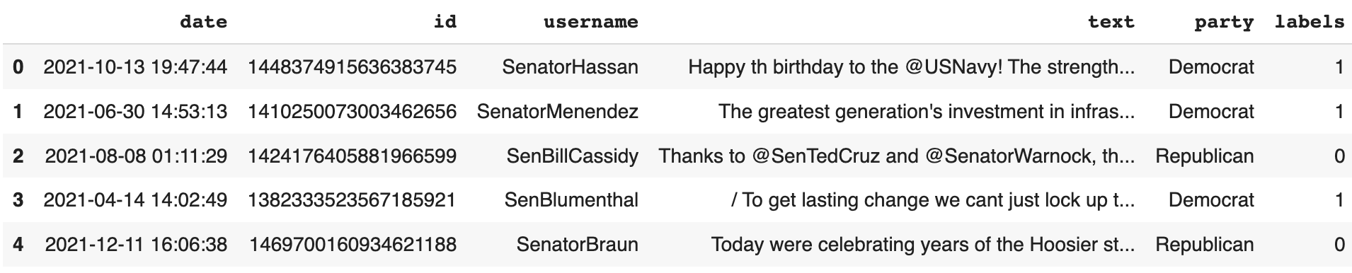
# Take a peak at the dataset
print(dataset)
dataset["train"].to_pandas().head()

Now we have an overview of the dataset:

DatasetDict({
    train: Dataset({
        features: ['date', 'id', 'username', 'text', 'party', 'labels'],
        num_rows: 79754
    })
    test: Dataset({
        features: ['date', 'id', 'username', 'text', 'party', 'labels'],
        num_rows: 19939
    })
})

And here's what the dataset looks like in dataframe form:

Step 3: Load the embedding model from the HuggingFace Hub

We will be using the Sentence Transformers all-MiniLM-L6-v2 model for this project for a few reasons. First, Sentence Transformers, in general, are models designed specifically for encoding sentences or text passages into embeddings. Second, we want to use a model small enough that we can embed our text using just a single GPU and store the results in memory. The all-MiniLM-L6-v2 model is a general purpose model that performs almost just as well as it's base model (all-mpnet-base-v2), but is significantly smaller and 5 times faster!

# Load the desired model
model = SentenceTransformer(
          'sentence-transformers/all-MiniLM-L6-v2', 
          device=device
)

Step 4: Generate the embeddings

Now it's time to generate the sentence embeddings. First, we need to create a function that generates embeddings for each split of the dataset. Notice that we split the data into batches to optimize the embedding process:

# Create function to generate embeddings (in batches) for a given dataset split
def generate_embeddings(split, batch_size=32):
    embeddings = []
    split_name = [name for name, data_split in dataset.items() if data_split is split][0]
    
    with tqdm(total=len(split), desc=f"Generating embeddings for {split_name} split") as pbar:
        for i in range(0, len(split), batch_size):
            batch_sentences = split['text'][i:i+batch_size]
            batch_embeddings = model.encode(batch_sentences)
            embeddings.extend(batch_embeddings)
            pbar.update(len(batch_sentences))
            
    return embeddings

Next, we generate the embeddings for each split and add them to their own new column in the dataset called embeddings:

# Generate and append embeddings to the train split
train_embeddings = generate_embeddings(dataset['train'])
dataset["train"] = dataset["train"].add_column("embeddings", train_embeddings)

# Generate and append embeddings to the test split
test_embeddings = generate_embeddings(dataset['test'])
dataset["test"] = dataset["test"].add_column("embeddings", test_embeddings)

This will take a few minutes, so feel free to grab yourself a cup of tea!

Step 5: Create a local Qdrant vector database

Because our dataset is split into train and test sets, we first need to combine them into a single dataset, which is quite simple:

# Combine train and test splits into a single dataset
combined_dataset = concatenate_datasets([dataset['train'], dataset['test']])

Now, we're ready to create our in-memory Qdrant instance. In this context, "in-memory" means that our vector database will be stored entirely within the system's main memory (RAM), instead of on a hard drive or in the cloud. This means that when we close the Colab notebook or restart it, the database will disappear.

# Create an in-memory Qdrant instance
client = QdrantClient(":memory:")

After instantiating the client, we create a collection for the embeddings to reside in. The size of each embedding refers to its dimensionality, or number of items inside the vector, which is always determined by the model. In our case, size is equal to 384, which is programmatically determined by model.get_sentence_embedding_dimension().

# Create a Qdrant collection for the embeddings
client.create_collection(
    collection_name="senator-tweets",
    vectors_config=models.VectorParams(
        size=model.get_sentence_embedding_dimension(),
        distance=models.Distance.COSINE,
    ),
)

Step 6: Upsert the embeddings into Qdrant

Finally, we are ready to upload the sentence embeddings of our dataset into our local Qdrant vector database.

Qdrant documentation recommends splitting up the dataset into batches, so we'll create a helper function for that and set our batch size:

# Create function to upsert embeddings in batches
def batched(iterable, n):
    iterator = iter(iterable)
    while batch := list(islice(iterator, n)):
        yield batch

batch_size = 100

And finally, we upsert our pre-generated embeddings to our Qdrant collection using the .upsert() method:

# Upsert the embeddings in batches
for batch in batched(combined_dataset, batch_size):
    ids = [point.pop("id") for point in batch]
    vectors = [point.pop("embeddings") for point in batch]

    client.upsert(
        collection_name="senator-tweets",
        points=models.Batch(
            ids=ids,
            vectors=vectors,
            payloads=batch,
        ),
    )

Exploring the data through search queries

Vector databases make downstream NLP tasks like clustering, question answering, and retrieval augmented generation (RAG), quick and effective.

For the purpose of this tutorial, we'll use our vector database for a simple task: semantic similarity search. Instead of keyword search, which matches specific words and phrases between search queries and potential results, semantic search embeds the search phrase with the same model as the embedded text and retrieves results based on the mathematical distance between their respective embeddings in the embedding space.

A simple search can find us the top 5 most relevant tweets related to immigration policy:

# Let's see what senators are saying about immigration policy
hits = client.search(
    collection_name="senator-tweets",
    query_vector=model.encode("Immigration policy").tolist(),
    limit=5
)
for hit in hits:
  print(hit.payload, "score:", hit.score)

And here's what our results look like:

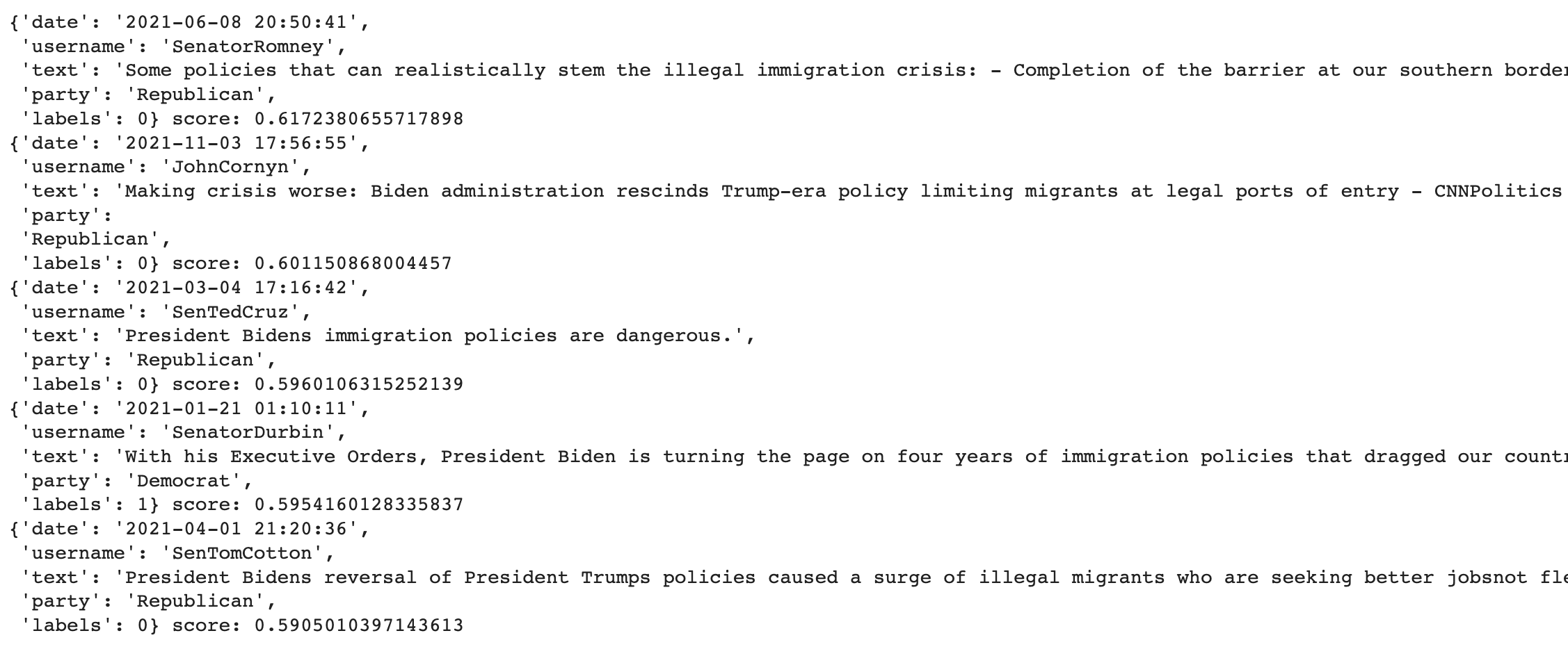
Most of these tweets are by Republican senators. If we want to see what the Democrats are saying about immigration policy, we can use the .Filter() method:

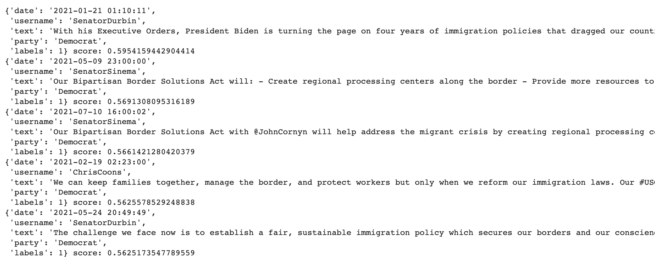
# Most of those tweets are by Republicans... let's see what the Dem's are saying
hits = client.search(
    collection_name="senator-tweets",
    query_vector=model.encode("Immigration policy").tolist(),
    query_filter=models.Filter(
        must=[
            models.FieldCondition(
                key="party",
                match=models.MatchValue(value="Democrat") # Filter by political party
            )
        ]
    ),
    limit=5
)
for hit in hits:
  print(hit.payload, "score:", hit.score)

Now, our results look like this:

There are many possibilities for further exploring this dataset, including using BERTopic to visualize the topics most prevalent among Democrats and Republicans, performing sentiment analysis on the tweets, or chaining the database with an LLM, like GPT-4 or Mistral 7B to ask questions about the dataset.

Summary

In this tutorial, we covered how to generate sentence embeddings for an existing dataset on the HuggingFace Hub, upsert those embeddings into a local Qdrant vector database, and explore the dataset using Qdrant's Python client. By seamlessly combining the capabilities of Sentence Transformers with the efficiency of Qdrant's vector database, we demonstrated a robust workflow for enhancing data exploration and retrieval that takes only 12 minutes set up!

If you're interested in learning more about vector databases, including how they work and what they can do, I recommend checking out Leonie Monigatti's excellent blog post, Explaining Vector Databases in 3 Levels of Difficulty.